Modeling with Nengo Part 1 - the Switching Observer

Disclaimer: The writing in this post is primarily a vehicle for my own learning and understanding, rather than an authoritative source of knowledge. Expect gaps and potential mistakes (please feel free to point them out!).

Introduction

On my journey to learn more about existing models that explain cognition, I wanted to explore the descriptive “Switching Observer” model described in a paper by Laquitaine & Gardner, 2018. My goal is to implement a simple neural circuit model in Nengo to simulate the neural population dynamics behind it.

The Paper

Laquitaine & Gardner set up a motion detection task where participants were shown a screen with moving circles and asked to estimate the direction of the moving circles after a stimulus direction was presented. For each trial, the circles initially moved in random directions. Then, a stimulus was presented where a percentage of the circles (termed ‘coherence’ in the paper) moved in a direction chosen by sampling from a Von Mises distribution (similar to a Gaussian distribution, but for angles).

The image below (Figure 1 from the paper) provides a good overview of the task setup. For each trial, a motion direction was sampled from a distribution with a mean of 225 degrees. The width of the distribution varied in blocks of trials. The coherence of the movement (6%, 12%, 24%) was randomly selected for each trial.

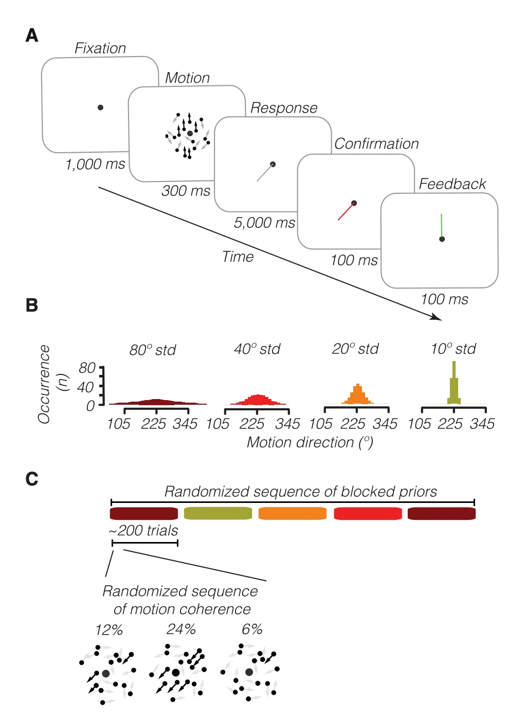
A key finding in the paper was that participant responses followed a bimodal distribution - there were two peaks. One mean was centered around the prior direction from which the stimulus motion direction was sampled, and the other was around the observed sensory evidence. This suggests that human motion detection doesn’t always fit a normative Bayesian model (i.e., integrating a prior belief with evidence to form a posterior probability). Instead, we may switch between our prior belief and what we observe as evidence.

Scope of this Post

Visual perception as switching rather than integrating? This is an intriguing finding. Does it imply there is a winner-takes-all mechanism at play?

In this series of posts, I aim to build up to a model neural circuit that emulates the switching behavior observed in the motion detection task.

In Part 1, I will first establish the basics of Nengo: generating inputs, creating populations of neurons, and implementing basic learning rules.

In Part 2, I will construct a simplified model of the switching observer in the context of a motion detection task. This model will simulate a population of neurons learning a prior from a series of observations and switching between prior and sensory evidence to make decisions on direction angles.

Implementation

Starting from a simple model that echoes a given signal, I will incrementally build up complexity in the Nengo model until we have a circuit that can learn the input signal using basic learning rules.

One Neuron

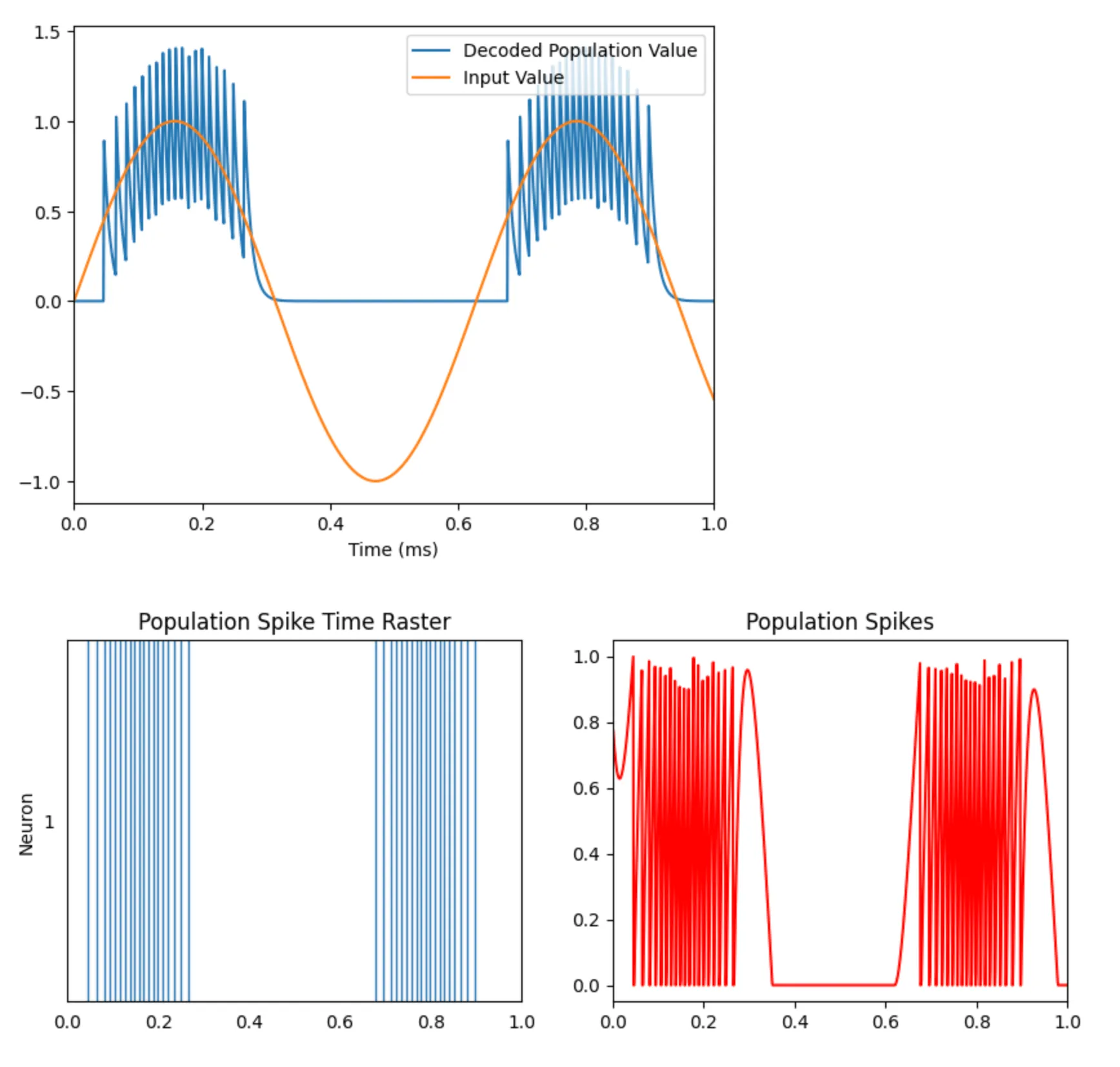
In this first section, we create an Ensemble with a single neuron and feed it a sine wave as input. In Nengo, the Ensemble abstraction is responsible for encoding information given to it in the underlying neurons’ spiking dynamics (we’ll explore the encoding/decoding process in a later post). We set up probes to monitor the input signal, the spike times for the single neuron, and the population spiking activity. These probes are used for plotting (code not shown here).

model = nengo.Network()
with model:
    input = nengo.Node(lambda x: np.sin(10*x))
    ensemble = nengo.Ensemble(
        1,
        # State space has a single dimension (i.e., a scalar)
        dimensions = 1,
        # Represents the range of values for the dimension
        intercepts = Uniform(-0.5, 0.5),
        # Neuron fires at a maximum rate of 100Hz
        max_rates = Uniform(100, 100),
        # N x M matrix where N = # of neurons, M = # of dimensions of input space.
        # This represents how inputs are converted into neuron representational space.
        encoders = [[1]],
    )

    nengo.Connection(input, ensemble)

    # Set up probes
    input_probe = nengo.Probe(input)
    # The raw spikes from the neuron
    spikes = nengo.Probe(ensemble.neurons)
    # Subthreshold soma voltage of the neuron
    voltage = nengo.Probe(ensemble.neurons, "voltage")
    # Spikes filtered by a 10ms post-synaptic filter
    filtered = nengo.Probe(ensemble, synapse=0.01)

with nengo.Simulator(model) as sim:
    sim.run(1) # 1 second

We observe that the single neuron population spikes (with increasing frequency) when the sine wave takes on higher values but ceases to spike for zero and negative values. With a single neuron, we are only able to encode the positive values of the input.

A Population of Neurons

The next step is to leverage a population of many neurons in the encoding/decoding of the sine input. This will give the model sensitivity to different directions of the input (i.e., the negative values) and more granularity when the model performs a linear weighted decoding.

Adding more neurons is a simple configuration change to the code we have above. We’ll use 10 neurons.

model = nengo.Network()
with model:
    input = nengo.Node(lambda x: np.sin(10*x))
    ensemble = nengo.Ensemble(
        10,
        dimensions = 1,
        max_rates = Uniform(100, 200),
        intercepts = Uniform(-0.5, 0.5),
    )

    nengo.Connection(input, ensemble)

    # Set up probes
    input_probe = nengo.Probe(input)
    spikes = nengo.Probe(ensemble.neurons)
    voltage = nengo.Probe(ensemble.neurons, "voltage")
    filtered = nengo.Probe(ensemble, synapse=0.01)

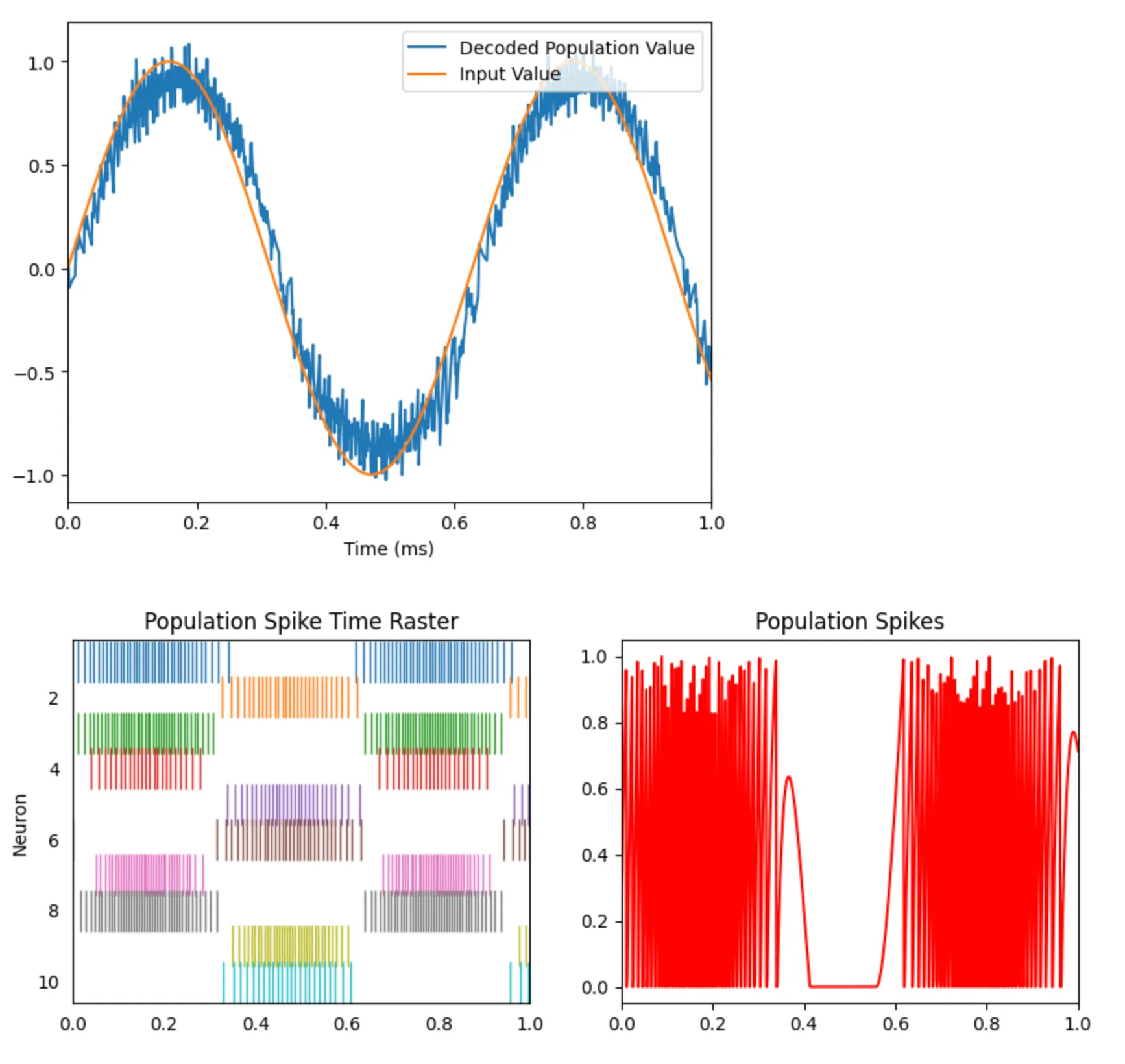
with nengo.Simulator(model) as sim:
    sim.run(1) # 1 second

Here are the updated plots. You can now see diversity in the spiking activity of the population - some neurons spike at positive values and others at negative values.

We are now able to decode the sine wave accurately!

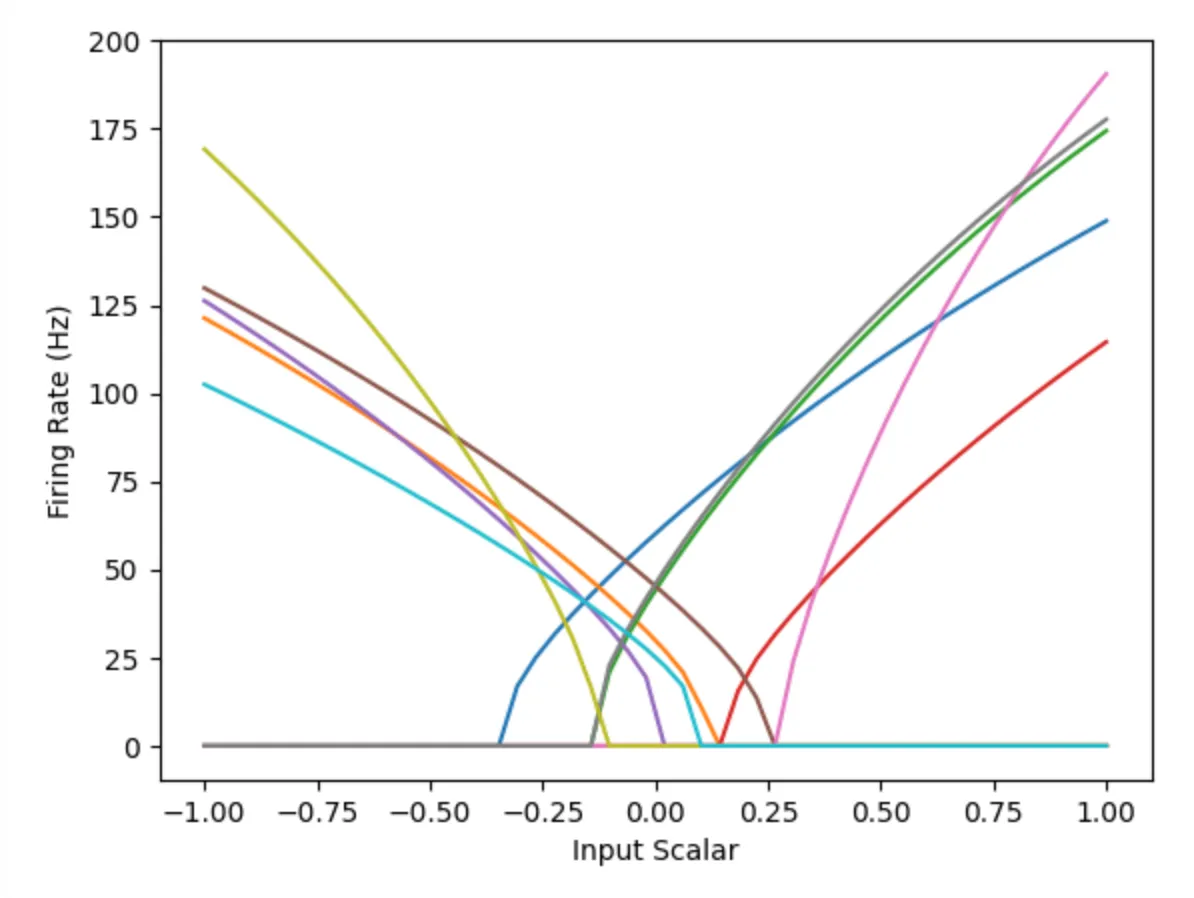
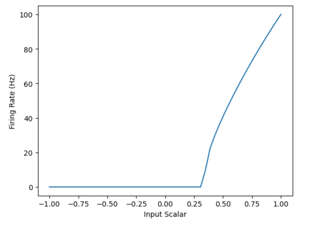
Looking at the Tuning Curves

Nengo allows us to plot the tuning curves of the various neurons in the population. This enables us to see what input values a particular neuron is sensitive to. Compare the first chart to the second, which captures the tuning curve for the population with one neuron. Notice how the population with many neurons can cover the whole input space, while the population with one neuron only covers values from 0.25 upwards.

Learning an Input

The final part of this post will focus on building a network that learns the structure of the input by leveraging an error connection as feedback.

The basic structure of this network is as follows:

• Input signal with a sine wave
• A pre ensemble that is fed the sine wave directly
• A post ensemble that will learn the structure of the input passed to it by the pre node
• An error ensemble that will compute the difference between pre and post and feed that to a learning rule connection with the post node.

model = nengo.Network()
with model:
    input = nengo.Node(lambda x: np.sin(10*x))
    pre = nengo.Ensemble(
        10,
        dimensions = 1,
        max_rates = Uniform(100, 200),
        intercepts = Uniform(-0.5, 0.5),
    )
    post = nengo.Ensemble(5, dimensions = 1)
    error = nengo.Ensemble(20, dimensions = 1)
    error_p = nengo.Probe(error, synapse=0.03)

    nengo.Connection(input, pre)
    pre_post_conn = nengo.Connection(pre, post, function = lambda x: rng.random())

    # Error = actual - target = post - pre
    nengo.Connection(post, error)
    nengo.Connection(pre, error, transform=-1)

    pre_post_conn.learning_rule_type = nengo.PES()
    nengo.Connection(error, pre_post_conn.learning_rule)

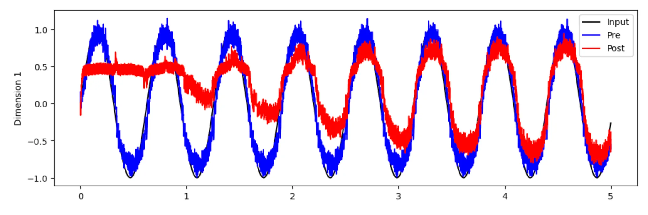
    # Set up probes
    input_probe = nengo.Probe(input)
    pre_spikes = nengo.Probe(pre.neurons)
    pre_decoded = nengo.Probe(pre, synapse=0.01)
    post_spikes = nengo.Probe(post.neurons)
    post_decoded = nengo.Probe(post, synapse=0.01)

with nengo.Simulator(model) as sim:
    sim.run(5.0) # 5 seconds

Below, we plot the decoded values on both nodes and see that over time, the post node learns the structure of the input.

Next Steps

In the next post, I’ll attempt to combine the fundamentals of Nengo with the switching observer model from the Laquitaine & Gardner paper.